Model-Based Analysis: First Steps
Autofill Values for Model Parameters
Add a further, copy and delete a model
1. How to open an existing project or create a new project and import data see Getting Started.
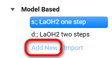
Add a New Model
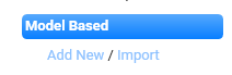
2. Add a new model, press Add New in the Project tree on the left panel:
3. Enter an optional Description of the model:
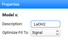
The Model Name (here “s”) will be defined automatically dependent on the reaction steps defined.
Set Optimize Fit to . It is set by default to Signal. It means that for the model-based analysis, the fitting of the experimental data and optimization of the parameters is done for the signal data. Conversion is recommended for projects of type DSC Curing, where the glass transition temperature should be predicted.
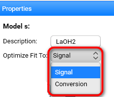
Note: the selection of Optimize Fit to is independent of the choice of how the data are displayed on the y-axis (see Ribbon Toolbar).
Define the Reaction Steps
4. Define the Reaction Steps using the icons:
![]() Add competitive step
(split step).
Add competitive step
(split step).
![]() Add consecutive step.
Add consecutive step.
![]() Remove step.
Remove step.
Example 1:
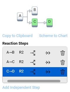
The reaction steps A→B and A→C are competitive steps, C→D is a consecutive step.
Click into the corresponding line (here marked in blue) in order to insert or remove reaction steps.
Example 2:
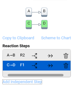
The independent steps C→D was created by clicking Add Independent Step.
Copy to Clipboard allows for exporting the illustration of the model to the clipboard - for example in order to insert it into a report.
Scheme to Chart is for adding the model scheme and the summary of the model steps to the chart as movable, editable text elements.
5. Define the Reaction Type for each individual reaction step (click the corresponding line in order to select the step, see Example 2 above). Not all reaction types are shown at once, use vertical scroll bar to see the rest of them:
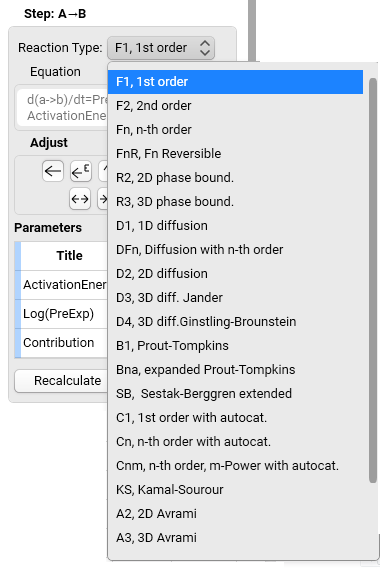
There are various reaction types possible (for details, see Reaction Types). Changing of the reaction type keeps the values for activation energy and pre-exponential factor, while other values are filled with pre-defined values, e.g.,n = 1.
The equation of the selected reaction step is shown in the panel.
Adjust a Reaction Step
6. If it is necessary, you can Adjust each individual reaction step:
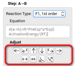
Use the arrows in order to manually move the calculated model curve closer to the experimental data. This procedure improves the start conditions for automatic calculations.
See more at Adjusting Arrows.
Optimize a Reaction Step
7. Optimize each individual reaction step:
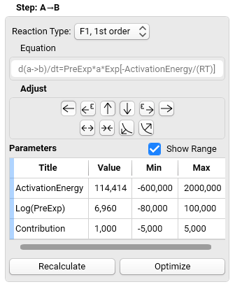
Click Optimize and the software will optimize the parameters Activation Energy, Pre-Exponential and Contribution for the selected reaction step.
Recalculate is for recalculation of the model curves with the actual parameters for the reaction step selected; those can be typed in manually for visual optimization.
Min and Max values, which can be displayed when checkbox Show Range is selected, may be adapted in order to limit the range of each parameter.
Autofill Values for Model Parameters
Some parameters belong not to the individual step, but for the total model. These parameters are the effect of total process like total peak area (DSC), total mass loss (TG), total length change (DIL), step height in logarithm of viscosity (Rheology) or step height in logarithm of ion viscosity (DEA).
The values of these parameters are present in the column Value in the table for the corresponding measurement. Initial values are taken from experimental data for each measurement.
The values in the table can be changed individually or all together by using the commands from AutoFill section.
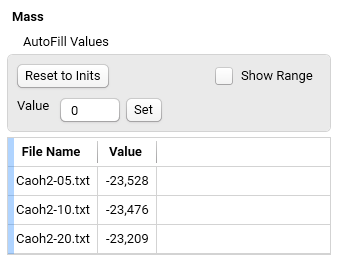
Resets to Inits: Sets the values in the table to the total effect (total peak area or total mass loss) from the experimental data.
Value - Input field - Set: Sets the Values in the table to the value typed in the Input field.
Show Range: shows the columns Min and Max in the table. During optimization of the model the optimized value of parameter must be stay between Min and Max values.
Min - Input field - Set: Sets the Min in the table to the value typed in the Input field.
Max - Input field - Set: Sets the Max in the table to the value typed in the Input field.
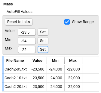
This table contains Value, Min and Max, which are set by Autofill function.
Optimize Model
8. Optimize or Recalculate model in Model Operations:
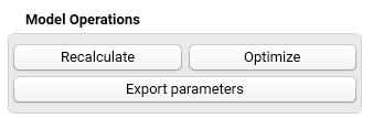
When each individual step has been adjusted and optimized, click Optimize button in Model Operations at the bottom of the Properties panel. The software will optimize all model parameters for best agreement between calculated curves and experimental data. The level of agreement is expressed by the Correlation coefficient R (see Statistics).
Recalculate is for recalculation of the model curves with the actual parameters for the reaction steps; those can be typed in manually for visual optimization.
The calculated effect of each step is shown (here: mass loss) and the model parameters can be seen for each individual reaction step.
Of course, Reaction Steps can be inserted or modified, and reaction types can be changed at any time. Press Recalculate and Optimize for updating the modeling.
Export Parameters
9. Export Parameters (after the model has been optimized):
Click on Export Parameters in Model Operations at the bottom of the Properties panel (screenshot above) and select the file name and location.
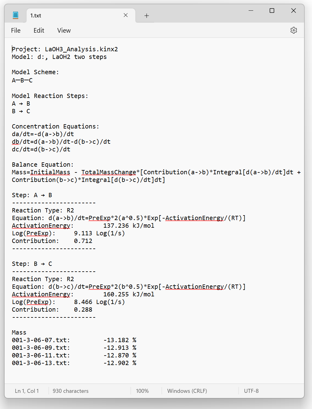
The model parameters and equations can be exported in a defined ASCII (.TXT) file:
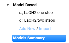
Models Summary
10. For a statistical summary and comparison of the models used and also regarding model-free analysis carried out, click at Models Summary:
You will see a table with all model-free and model-based models you have clicked in this project before:

See Statistics for further details.
Add, Copy or Delete a Model
11. It is possible to add, copy, or delete a model. To add a new model just click on Add New in Model Based section of Project Tree:
To copy, export to a file or delete a model just right-mouse-click of the model in Project tree:
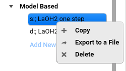
In the context menu select option you want.
Export / Import a Model
12. One can also export a model to a KINX-MODEL binary file. Sometimes it is important to share the model with your colleagues. They can import such exported file into their Kinetics Neo projects.
To export a model select it in the Project tree and make right-mouse-click on it (screenshot above). Select option Export to a File .
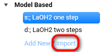
To import a model from the file click on Import in Model Based section of the Project tree:
A model can be used independent of the data type.