Predictions: Isothermal Lifetime

Prediction of the times at which defined conversion values are reached for different isothermal temperatures:

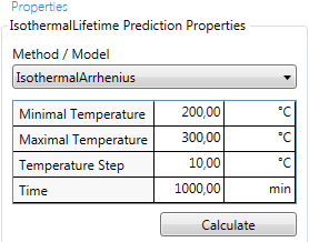
First, a Method/Model (model-free or model-based) needs to be selected (here: Isothermal Arrhenius), where only those models are offered with which the data were already analyzed.

• The Minimal and Maximal Temperatures define the minimum and maximum isothermal temperatures. Default values are suggested by the software according to the experimental data. Of course, the Minimal and Maximal Temperatures can be set to values that are not covered by experimental data.
• Temperature Step defines the difference between each isothermal temperature.
• Time is the maximum time of the simulation. The time value must be long enough to reach the desired degrees of conversion.

Isoconversion Curves can be shown by selecting All, None, Default or Custom. In case of the model Isothermal Arrhenius, the simulated curve is restricted to one line: time-to-event.

Press Calculate for calculations/update of calculations.

Exemplary results:

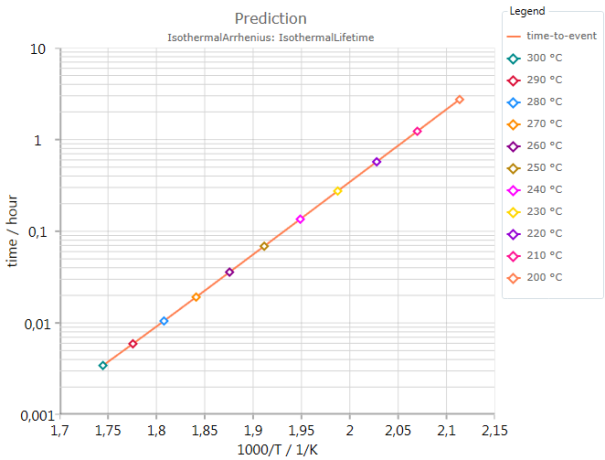
This example is about the prediction of so-called oxidation induction times (OIT). A simulated isoconversion curve for time-to-event is shown as a function of the inverse isothermal temperatures. This curve reflects the times to reach oxidation induction for different isothermal temperatures.

A second example depicts simulated isoconversion curves for the isothermal crystallization of a polymer:

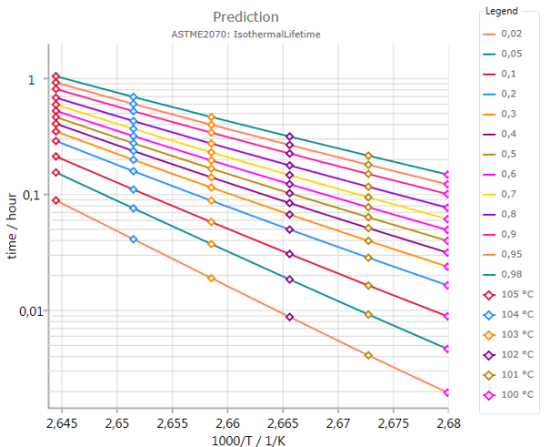
In this case, the time to reach a conversion value is the faster the lower the isothermal crystallization temperature is.

Customization and exporting of the results can be done via Ribbon Toolbar.